By Eben van Tonder, 14 September 2026

Executive Summary
The goal behind this system is a dry salted beef omasum product that reaches its export markets without refrigeration at any point after it leaves the drying room. The production system that delivers that product, cleaning, salting, pressing, drying, and packing, is set out in full in the companion guide, Dry Salted Beef Omasum Production, published at earthwormexpress.com/the-meat-factory/meat-science-research/dry-salted-beef-omasum-production [10]. That guide treats ambient shelf stability as the outcome of several preservation factors working together, commonly called hurdle technology, rather than any single step doing the whole job on its own. Salt content, an acid wash, potassium sorbate against mould, and a moisture-barrier pack each contribute one hurdle. Drying is another, and it is the hurdle this document exists to measure, because none of the other hurdles compensate for a piece that has not actually been dried down to the working water activity target at its thickest, slowest-drying point. A piece that looks dry on the outside but is still wet at the root has not cleared this hurdle, regardless of how it looks or how the other hurdles are set, and the shelf-stable claim for that batch depends on knowing whether it has, not assuming it has.
Confirming that reliably, on every batch, at a sample count large enough to catch the worst location rather than an average, is not possible without a working water activity measurement system in the plant. That need is what drives the choice, set out below, between an expensive commercial meter and a low-cost chamber built in-house, and why the sample count per batch has to be adequate rather than convenient.
What to Buy
Two categories of equipment are needed, not one. The first is a single commercial reference instrument, a Novasina LabStart or equivalent, roughly 1,700 euros, bought once. The second is a set of DIY chambers, each built for roughly 150 to 200 euros from the parts listed later in this guide, a Sensirion SHT85 or Adafruit SHT31-D sensor, an Adafruit Feather HUZZAH microcontroller, an OLED display, and a MicroSD data logger, sealed into a glass jar. A starting set of three DIY chambers with spares, alongside the one reference instrument, comes to roughly 2,300 to 2,700 euros as a total starting outlay.
What Will Be Done
The reference instrument calibrates and validates the DIY chambers during setup, confirming that the cheap sensors, once corrected, agree with a trusted method on actual omasum samples. Once that agreement is demonstrated, the DIY chambers become the daily workhorse, run in parallel, a chamber at a time or several at once, to screen 10 to 15 samples per one tonne batch during drying. Each reading logs automatically to a MicroSD card with a sample ID, a time to plateau, and a corrected aw. A batch is released once every sample in that set meets the target aw, not once the average does.
Why Two Kinds of Instrument, Not One
A DIY chamber built from a 15 euro sensor is only as trustworthy as the calibration behind it. The reference instrument is what that calibration is checked against, and it continues afterward as a working meter in its own right, available whenever a result needs to be trusted without depending on a chamber that has not been recently checked. Running DIY chambers without ever validating them against a reference instrument would mean trusting a correction line that has never been tested against anything beyond two salt slurries. Running only the reference instrument, without the DIY chambers, would mean paying roughly 1,700 euros for every additional chamber needed to screen a growing volume of batches, instead of roughly 150 to 200 euros. The two together, one trusted anchor and several cheap workhorses checked against it, is what makes daily testing at the sample count this product needs financially realistic.
The Money Saver, in Outline
Matching the validation capacity of one reference instrument plus three DIY chambers using commercial units alone would cost three to four times as much, since each additional commercial unit runs close to the reference instrument’s own price, while each additional DIY chamber costs a small fraction of that. This is set out in full in the Economic Review section near the end of this guide, alongside the separate and larger saving available from selling omasum as a shelf-stable, ambient product rather than a refrigerated one.
What a Shelf-Stable Product Is Worth at Container Scale
Eben van Tonder has estimated the saving from selling shelf-stable, ambient omasum rather than a refrigerated equivalent at approximately 13 euro cents per kilogram. This figure is the working estimate used for this guide and has not been independently broken down or sourced here into its component parts, freight, cold storage, and spoilage risk among them. On a 28 tonne container, 28,000 kilograms, that comes to a saving of approximately 3,640 euros per container. Against a container sold at 5 euros per kilogram, a total sale value of approximately 140,000 euros, that saving represents approximately 2.6 percent of sale value. A 2.6 percent margin improvement on a commodity trade, achieved without changing the product’s formulation or selling price, is a meaningful figure, not a marginal one.
Other Benefits of Ambient Stability
Beyond the direct per kilogram saving, a shelf-stable product removes several risks that a refrigerated product carries. Reefer freight itself commands a structural premium over dry container rates, commonly 50 to 100 percent above the equivalent dry rate on the same route, a premium that persists in stable markets and is not simply a symptom of tight capacity [7]. An ambient product avoids this premium entirely, avoids dependence on functioning reefer plugs at every port and transhipment point along the route, avoids the total loss risk of a single refrigeration failure during a multi week ocean voyage, and can be warehoused and distributed in markets, including much of West Africa, where a reliable cold chain cannot be assumed all the way to the point of sale.
Why the Exact aw Target Is Not Optional
None of these benefits are available for free. Drying is one hurdle among several in this product’s preservation strategy, working alongside the acid wash and the salt content from dry salting itself, but it is the hurdle that does the specific job of denying microorganisms free water [5][6]. If the finished aw sits above the working target, the product is not actually shelf stable regardless of how it looks or weighs, and the entire economic case above, the avoided reefer premium, the avoided cold chain risk, the wider market reach, collapses along with it. If the aw is pushed too far below target in an attempt to be safe, the product suffers case hardening and yield loss for no food safety benefit. The measurement system described in this guide exists because the target aw, not a guess at it, is what the rest of this document’s economic case depends on.
Water Activity Versus Moisture Content
AW Versus Moisture Content, in Simple Terms
Moisture content, expressed as percentage of water lost during drying, tells you how much water has left the product. It does not tell you how much of the water still inside is actually available to a bacterium, yeast, or mould cell. Salt, sugar, and protein all bind some of that remaining water tightly enough that microorganisms cannot use it. Water activity, aw, measures only the free, usable fraction, on a scale from 0 to 1. Two pieces of omasum can lose the same percentage of weight during drying and still sit at different water activities, because one had more salt working on the water that remained. This is why a weight loss figure alone, without a corresponding water activity reading, cannot tell you whether a piece is actually safe to release.
What Water Activity Actually Measures
Formally, water activity is the ratio of the vapour pressure of water in the product to the vapour pressure of pure water at the same temperature. A reading of 1.0 means the water in the product is behaving exactly as pure, unbound water would, an open dish of water sitting in the room. Nothing in the product is holding onto it, so it exerts its full vapour pressure and will equilibrate with the air around it at 100 percent relative humidity. Fresh, undried meat sits close to this figure, typically around 0.98 to 0.99, because almost none of its water is yet bound tightly enough to change that behaviour.
As aw falls below 1.0, progressively more of the remaining water is bound, to dissolved salt ions, to sugars, to protein surfaces, or held in increasingly narrow spaces within the tissue, and progressively less of it is free to escape into the vapour phase. This is not a bookkeeping distinction. It is the same physical property the sealed jar chamber in this guide actually measures: a piece of omasum sealed into an airtight headspace will drive that headspace toward its own equilibrium relative humidity, higher for a wetter, less bound piece, lower for a drier, more heavily salted one, and the reading only stabilises once the vapour pressure of the sample and the vapour pressure of the air above it have equalised. A lower aw means the product releases less moisture into surrounding air and draws moisture in more readily from humid air, which is also why an under-specified pack in a humid destination market can let a properly dried piece pick up water again after release, as the companion production guide sets out.
The relevance to microorganisms follows directly from the same physics. A bacterium, yeast, or mould cell takes up water across its membrane by relying on a favourable gradient between the water activity outside the cell and the more concentrated solution inside it. As the surrounding aw falls, that gradient narrows, and once it falls far enough, the direction can reverse, so that water is pulled out of the cell rather than into it, exactly as concentrated brine draws water out of tissue by osmosis elsewhere in this guide. Each organism group has a characteristic minimum aw below which it can no longer draw in enough water to grow, which is why the threshold table above lists a descending sequence of limits, spoilage bacteria first, then most pathogens, then yeasts, then ordinary moulds, and finally the xerophilic moulds that tolerate the least available water of any organism group studied. A single aw reading therefore tells you, directly, which of these groups are still able to function in that piece of omasum and which have already been shut out, in a way a moisture percentage cannot.
This is also why moisture content is not a suitable substitute measurement, not merely a less convenient one. Water content reports the mass of water present without distinguishing free water from bound water, so two products can share an identical moisture percentage while sitting at very different water activities, depending on what else is dissolved in that water, exactly as the biltong data below demonstrates for two styles of the same product. The distinction was first established, not assumed, by the Australian microbiologist William James Scott, whose 1953 studies of Staphylococcus aureus and related organisms showed that microbial growth in food correlates with water activity rather than with total water content, a finding that reshaped how food safety has been assessed ever since [9]. Every threshold cited in this guide traces back to that same distinction.
The Relationship Between aw and Actual Water Content
There is no single formula that converts a moisture percentage into an aw value across different products. The relationship, known formally as a moisture sorption isotherm, depends on what else is in the product competing for that water, principally salt, but also protein and any sugar present, and it is specific to each formulation rather than universal. The commercial biltong data already cited illustrates this directly rather than abstractly. Dry biltong at 21.5 to 25.3 percent moisture measured aw 0.65 to 0.68, while moist biltong at roughly double that moisture, 35.1 to 42.8 percent, measured aw 0.85 to 0.89 [2]. The moisture roughly doubled, but the aw did not follow it proportionally, because the dry style also carried a higher salt content, 5.5 to 7.9 percent against 3.8 to 5.6 percent in the moist style, and that additional salt binds a disproportionate share of the remaining water [2]. A separate biltong drying study found a comparable pattern at intermediate points, aw above 0.81 at roughly 50 percent weight loss falling to aw below 0.78 at roughly 65 percent weight loss, a relationship that flattens rather than tracks moisture loss linearly as drying continues [4]. The practical consequence is that a moisture percentage alone cannot substitute for an aw reading on omasum, and any moisture target used as a proxy during production should be established empirically for this specific formulation, salt rate included, rather than assumed from a generic drying curve or from biltong’s own figures directly.
Why Water Activity Is the Target, Not Moisture Loss
Water activity is the target because it is the figure that actually governs whether microorganisms can grow, not the figure that governs how the product looks or weighs. It addresses several distinct organism groups, each with its own threshold, so a single aw reading tells you which of these risks are still active and which have already been shut down. The threshold values below are drawn from the standard review of water activity and microbial growth in the food science literature [1].
| Water activity | What stops growing at or below this level |
| Below 0.91 | Most spoilage bacteria |
| Below 0.87 | Most pathogenic bacteria, including Salmonella and E. coli |
| Below 0.88 | Most yeasts |
| Below 0.86 | Staphylococcus aureus, a notable exception among pathogens because it tolerates lower water activity than most other bacteria of concern |
| Below 0.80 | Most ordinary moulds |
| Below 0.70 | The point generally described as the practical limit for common spoilage yeasts and moulds |
| Below 0.65 down to about 0.60 | Xerophilic, dry tolerant moulds, the most resistant fungal group and the last one to be shut down as a product dries |
| Below 0.60 | The generally accepted floor below which no microbial growth of any kind occurs |
Water activity (aw) also addresses yeast and mould directly, and is in fact the figure that governs them specifically, since bacteria are usually the first risk eliminated as a salted product dries, while yeast and then mould, ending with the more resistant xerophilic strains, are what determine how far drying actually needs to go.
Setting the Drying Target
Drying and Product Quality
A target of aw 0.60 to 0.65, taken purely from the microbial threshold table, says nothing about what that level of dryness does to the tissue and to the eating quality of the finished product. Commercial precedent from biltong, the closest documented South African analogue to omasum, does not support drying that far.
What Commercial Biltong Measures
A peer reviewed study of commercial South African biltong samples found two distinct categories rather than one target figure [2]. Dry biltong measured aw 0.65 to 0.68, with moisture content between 21.5 and 25.3 percent. Moist biltong, the more widely preferred style, measured aw 0.85 to 0.89, with moisture content between 35.1 and 42.8 percent [2]. Biltong as a category is classified as an intermediate moisture food falling across the range aw 0.60 to 0.90, and consumer preference studies cited in a review of South African biltong processing found that consumers generally prefer the higher moisture, higher aw style over the drier one [3].
The actual commercial range in South Africa therefore sits well above the 0.60 to 0.65 figure proposed earlier, even for the drier style, and the more popular moist style sits close to double that water activity. A target of 0.60 pushed on omasum would be drier than the driest commercial biltong on the market, not merely at the safe end of it.
Drying and Tissue Damage
For a thick or folded tissue such as omasum, aggressive drying carries a specific structural risk called case hardening, where the outer surface dries and stiffens quickly while moisture is still migrating out from the interior, trapping that interior moisture behind a dense, leathery crust rather than letting it escape evenly. This produces a piece that is dry and even brittle at the surface while the core has not actually reached target, and it also produces a texture that resists rehydration later, since the hardened outer layer restricts water uptake during cooking. No study measuring this specifically on omasum has been found, so this is a reasoned expectation drawn from general dehydration behaviour in thick collagenous tissue, not a cited omasum specific finding, and it is a further reason not to chase the lowest aw the microbial threshold table alone would suggest.
Do Not Rely on Drying Alone
The answer is hurdle technology, the practice of combining several smaller preservation barriers rather than pushing any single one to an extreme [5][6]. Biltong itself is a working example. Its marinade lowers pH with vinegar, its salt content sits high, at 5.5 to 7.9 percent in the dry style and 3.8 to 5.6 percent in the moist style, and its spice blend, typically coriander and pepper, contributes further antimicrobial activity on top of the acid and the salt [2]. Ground biltong challenged with mould isolates showed no meaningful mould development over two months of storage at 25 degrees Celsius when the aw was held at 0.70, though limited growth was still noted at aw 0.72, 0.78, and 0.80, precisely because the acid, salt, and drying were working together rather than the drying carrying the full burden alone [3].
What This Means for the Omasum Target
The earlier recommendation of aw 0.60 to 0.65 for a year of ambient shelf life should therefore be adjusted. A target closer to 0.70, in line with both the biltong mould challenge result and the general literature review recommendation of drying to aw 0.70 to 0.75 to prevent microbial growth, is better supported by real product precedent, provided it is not asked to do the job alone. The organic acid wash already built into the process, and the salt content from dry salting itself, are both hurdles in this same sense, and their contribution should be counted alongside the final aw target rather than treated as separate from it. If year round ambient stability at aw 0.70 rather than 0.60 needs an additional margin, that margin should come from strengthening one of the other hurdles, a stronger acid wash, a higher salt percentage, or the potassium sorbate treatment already specified for the drying stage, rather than from drying the omasum harder than commercial biltong ever is.
The Target for a Year of Ambient Shelf Life
If the goal is stability for a full year without refrigeration, the practical limit of aw 0.70 is not a safe target on its own, since xerophilic moulds are documented to grow down to roughly 0.60 to 0.65, well below that limit. A year long ambient shelf life needs a margin below the most resistant organism still capable of growth, not just below the point where ordinary spoilage yeast and mould stop. Aiming for an aw at or below 0.65, and ideally closer to 0.60, gives that margin. This is a reasoned engineering target built from the thresholds above, not a cited figure specific to omasum.
Sampling and Scheduling
How Many Samples From a One Tonne Batch
There is no published sampling plan specific to dry salted omasum, so this has to be reasoned from general food sampling statistics rather than cited from a study on this exact product. The starting point is that omasum is a heterogeneous tissue, folded, of varying thickness, with salt and moisture distributed unevenly, so a one tonne batch cannot be represented by a single sample regardless of how carefully it is chosen.
A practical starting design is 10 to 15 samples, taken from different locations within the batch, different thicknesses, different positions in the salting stack, different pieces rather than repeated cuts from the same piece. This is a reasoned starting point, not a statistically derived final number. The correct way to fix the final number is to calculate it from batch to batch variability once a handful of production runs have been logged. Once the standard deviation of aw readings across a batch is known, the standard sample size formula, n equals the square of Z times the standard deviation divided by the acceptable margin of error, gives a defensible sample count for the actual variability rather than a guess. Until that calculation has been done, 10 to 15 samples per tonne is the reasonable working figure to validate the target with, weighted toward the thickest and most folded sections, since those are the last parts of the batch to reach target and therefore the parts most likely to fail if the batch fails.
Relating AW, Date, Temperature, and Drying Time, Combined With the DIY System
Ambient temperature and humidity change through the year, and drying rate changes with them, so a drying schedule that reaches target in ten days in a dry, cool month may need longer in a humid, warm one. Building a log that records the date, the ambient temperature and humidity for each drying run, and the final validated aw for that batch, over enough cycles, allows prediction of how long a given batch will need to reach target under the conditions of that particular week, rather than running every batch to a fixed number of days regardless of the weather. This is a predictive tool, not a substitute for validation. It indicates when a batch is likely close to target so testing can start at the right time, not that the target has actually been reached.
This is where a cheap temperature probe becomes useful alongside the DIY aw chambers rather than instead of them. A basic digital probe thermometer, a few euros each, can be placed in multiple locations through the stack daily without needing to open a sealed aw chamber for every check, giving a live picture of how the drying is progressing across the whole batch at very low cost. Once the log and the probe readings suggest a batch is approaching the expected time to target for that week’s conditions, that is the signal to pull the statistically justified sample set, the 10 to 15 pieces discussed above, and run them through the calibrated DIY chambers to confirm the actual aw, rather than assuming the log’s prediction is correct. The probe and the log indicate when to test. The DIY chamber and its calibration are what actually confirm the result.
Choosing the Measurement Approach
Outline of the DIY Unit at a Fraction of the Cost
The unit specified for this project, a Sensirion SHT85 or Adafruit SHT31-D sensor, an Adafruit Feather HUZZAH microcontroller, an OLED display, and a MicroSD logging module, sealed into a glass jar with a silicone grommet feedthrough, costs roughly 150 to 200 euros to build, with a further 100 to 150 euros for a full spares set. This sits at roughly a tenth of the cost of even the cheapest new commercial entry level meter, and logs every reading automatically to a card with no network dependency, as set out in the build list and spares tables below.
Approximate Cost Comparison
The two routes are not alternatives to choose between. A reliable programme needs both, one commercial reference instrument to calibrate and validate against, and a set of DIY chambers built alongside it. The reference unit is bought once and used for both purposes, validating the DIY chambers during setup and then continuing to serve as a working meter for production checks afterward. The DIY chamber count starts small during validation and is scaled up once the daily screening volume is known.
| Item | Approximate cost | Notes |
| Reference instrument, Novasina LabStart or equivalent | Roughly 1,700 euros | Bought once. Serves as the calibration reference during validation and continues as a working meter for production checks afterward |
| DIY chambers built for the validation phase, 2 to 3 units | Roughly 300 to 600 euros | Based on 150 to 200 euros per chamber, run alongside the reference instrument so each sample can be read on both at the same time |
| Spares for the validation phase chambers | Roughly 150 to 300 euros | Covers the spare sensors, boards, jars, and wiring set out in the spares table, sized to 2 to 3 chambers |
| Additional DIY chambers for daily production screening, scaled to need | Roughly 150 to 200 euros per chamber | Added once validation confirms the method and the daily sample count is known. This is where the DIY approach keeps its cost advantage, since matching the same throughput with additional commercial units would cost roughly 1,700 euros per chamber instead |
A project built this way, one reference instrument plus three DIY chambers with spares, comes to roughly 2,300 to 2,700 euros as a starting total, before any scale up. Matching that same validation capacity with commercial units alone would cost three to four times as much, since each additional commercial unit runs close to the reference instrument’s own price, while each additional DIY chamber for the scale up phase costs a small fraction of that.
Why Calibration Requires Access to a Reference Instrument
A DIY chamber, however well built, only produces a defensible water activity figure once its sensor has been checked against known reference points and, ideally, against a validated commercial instrument reading the same sample. The salt slurry calibration already described establishes the sensor’s accuracy at two known points, but confirming that the whole chamber, sample preparation, and equilibrium algorithm together produce results that agree with a trusted instrument on the actual product, omasum, requires access to that instrument during validation.
Renting a commercial meter for the validation period is one option, and several laboratory equipment suppliers offer short term hire specifically for this kind of validation project. Buying one outright is the better route, because the unit does not become redundant once validation ends. It becomes the reference instrument used to calibrate and periodically check the DIY chambers going forward, and it also becomes a working meter in its own right, available to measure aw directly on production batches whenever a result needs to be trusted without depending on a chamber that has not been recently checked.
Reference Unit Options
| Instrument | Approximate price | Notes |
| Novasina LabStart | Entry level, commonly cited around 1,700 euros for a new unit | Covers the 0.20 to 0.80 aw range, which sits comfortably around the working target discussed above, uses a resistive electrolytic sensor, and is described as a low cost precision instrument aimed at exactly this kind of routine supervisory check rather than full laboratory reference work |
| Rotronic HygroPalm HP23-AW-A | Roughly 1,500 to 3,000 euros new, depending on kit configuration | A handheld unit covering the full 0 to 1.00 aw range, giving more flexibility if the same instrument is ever needed for products well outside the intermediate moisture range, such as fresh meat or wet cured products |
| Used Decagon or METER AquaLab Series 3 TE | Roughly 1,700 to 2,500 euros on the secondhand market | A chilled mirror dew point instrument, the more precise measurement principle discussed earlier, at plus or minus 0.003 aw, available at a lower cost than new but with the usual secondhand risk of unknown service history and no manufacturer warranty |
Given the working target established above, aw at or below 0.65, the Novasina LabStart’s stated range of 0.20 to 0.80 covers this comfortably, and its price point matches the figure already mentioned. The Rotronic is the more flexible instrument if the same unit will also be used on products outside this range. The used AquaLab offers the highest precision of the three but carries the usual risk of buying an instrument secondhand without a service record.
Building the DIY Chamber

Build List for One Unit
| Item | What to search or order | Quantity |
| Humidity and temperature sensor breakout | Sensirion SHT85 digital humidity sensor breakout board. Order from Mouser Electronics, Digi-Key, or Sensirion directly. If unavailable, the Adafruit SHT31-D breakout (Adafruit product 2857) is the easier to source substitute, slightly lower accuracy but the same working principle | 1 |
| Microcontroller | Adafruit Feather HUZZAH ESP8266 with headers, Adafruit product 3046 (or the loose header version, product 2821, which needs the headers soldered on separately) | 1 |
| Display module | 0.96 inch I2C OLED display module, SSD1306 driver, 128 by 64 pixels. Widely sold under this exact description on Amazon, AliExpress, or via Conrad Electronic in Austria | 1 |
| Data logging module | MicroSD card breakout board with SPI interface, sold as “MicroSD card module SPI” or “Micro SD card breakout board”, available from Adafruit, SparkFun, or Conrad Electronic, paired with a small MicroSD card, 8 GB is more than sufficient for daily CSV logs | 1 module, 1 card |
| Connecting wires | Female to female jumper wires, 20 centimetre length, a pack of at least 10 | 1 pack |
| Cable feedthrough | Silicone rubber cable grommet, 6 to 8 millimetre bore, sold as “silicone wire grommet” or “cable entry grommet” | 3 |
| Sealant | Food grade silicone sealant, a small tube, sold as “aquarium safe” or “food grade” silicone sealant | 1 tube |
| Drill bit | Step drill bit or a standard twist bit sized to match the grommet, for making the hole in the jar lid | 1 |
| Jars | Wide mouth glass mason jars with two piece metal lids, 500 millilitre size, Ball or Kilner brand or the equivalent sold locally | 3 |
| Power source | USB power bank, small capacity, around 5,000 mAh, with a micro USB output | 1 |
| USB cable | Micro USB charging and data cable, standard length | 1 |
| Enclosure for electronics | Small IP65 rated ABS project box, dimensions to fit the Feather board, display, and SD card module, sold as “waterproof project enclosure box” | 1 |
| Calibration salt, sodium chloride | Sodium chloride, ACS reagent grade, from a laboratory chemical supplier such as Carl Roth, VWR, or Sigma Aldrich. Reagent grade rather than ordinary table salt, since additives in table salt such as anti caking agents and iodine can shift the reference value away from the certified 0.753 | 250 grams |
| Calibration salt, potassium chloride | Potassium chloride, ACS reagent grade, from the same supplier as above | 250 grams |
| Distilled water | Distilled or deionised water, sold in bottles at any hardware or pharmacy | 1 to 2 litres |
| Small calibration jars | Small glass jars with airtight lids, 100 to 200 millilitre size, for holding the salt slurries separately from the field jar | 2 |
| Labels | Waterproof marker and small adhesive labels, for identifying which jar holds which slurry or sample | 1 set |
| Soldering iron and solder | Basic soldering iron kit with lead free solder, needed only if the headers on the Feather board are not pre soldered | 1 kit |
Spare Parts, With the Reason Each Is Likely to Fail
| Part | Why it is at risk | Spare quantity to buy |
| Glass jars | Glass cracks or breaks during handling in transit and during repeated daily use in the field | 3 additional, so 6 total |
| Sensor breakout board | The sensing element is delicate, can be damaged by physical shock, direct contact with moisture if the grommet seal fails, dust ingress, or static discharge during handling | 1 additional |
| MicroSD card and breakout module | Card contacts corrode in humid climates, and cards fail after repeated read and write cycles or physical wear from being pulled out daily | 1 additional card, 1 additional breakout module |
| Jumper wires | Connectors loosen and corrode in humid climates, and repeated opening and closing of the jar strains the wire where it passes through the lid | 1 extra pack |
| Silicone grommets | Silicone tears or loses its seal with repeated threading of the wire through it | 3 additional |
| Silicone sealant tube | A tube left partly used can dry out and harden before the next application is needed | 1 unopened spare tube |
| Micro USB cable | Cables fray and break at the connector with repeated use and travel | 1 additional |
| USB power bank | Batteries degrade with heat exposure, and a single power bank leaves no backup if it fails or is lost | 1 additional |
| OLED display module | The screen is thin glass and cracks easily if the enclosure is dropped or crushed in transit | 1 additional |
| Microcontroller board | Less likely to fail outright, but humidity, dust, or a power surge can damage it, and there is no easy local replacement in the field | 1 additional, pre configured with the same code before travel |
Complete List, Build Items and Spares Combined
| Item | Quantity for the build | Quantity as spares | Total to buy |
| Sensirion SHT85 breakout board (or Adafruit SHT31-D) | 1 | 1 | 2 |
| Adafruit Feather HUZZAH ESP8266 (assembled, with headers) | 1 | 1 | 2 |
| SSD1306 OLED display module | 1 | 1 | 2 |
| MicroSD card breakout module and card | 1 | 1 | 2 |
| Female to female jumper wire pack | 1 | 1 | 2 |
| Silicone cable grommets | 3 | 3 | 6 |
| Food grade silicone sealant tube | 1 | 1 | 2 |
| Step drill bit | 1 | 0 | 1 |
| Wide mouth glass jars, 500 ml | 3 | 3 | 6 |
| USB power bank, 5,000 mAh | 1 | 1 | 2 |
| Micro USB cable | 1 | 1 | 2 |
| IP65 project enclosure box | 1 | 0 | 1 |
| Sodium chloride, ACS reagent grade | 250 g | 0 | 250 g |
| Potassium chloride, ACS reagent grade | 250 g | 0 | 250 g |
| Distilled water | 1 to 2 litres | 0 | 1 to 2 litres |
| Small glass calibration jars, 100 to 200 ml | 2 | 0 | 2 |
| Waterproof marker and labels | 1 set | 0 | 1 set |
| Soldering iron kit with lead free solder | 1 | 0 | 1 |
Sourcing the Parts
Source the electronics, including the MicroSD card breakout for the data logger, from Conrad Electronic, Mouser, Digi-Key, or Adafruit directly, all of which ship to Austria. Source the reagent grade salts from Carl Roth or VWR, both established Austrian and German laboratory suppliers, because a supermarket product would leave the calibration reference values open to question. The jars, sealant, drill bit, and cabling remain ordinary hardware and kitchenware items, available locally or through Amazon.at.
System Architecture and Components

Physical Assembly Breakdown
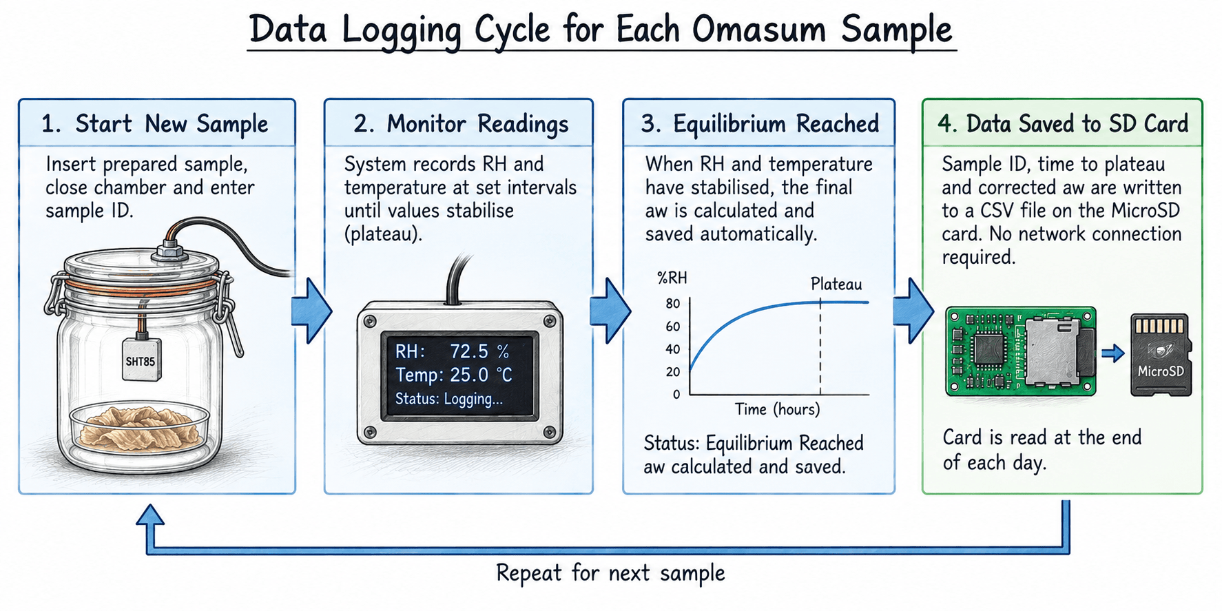
- Airtight Chamber. A small glass jar or plastic vial with a rubber gasket seal. Keeping the headspace volume minimal reduces the time required to reach vapor equilibrium.
- Capacitive RH/T Sensor. An SHT85 or similar digital sensor suspended near the top of the container, avoiding direct contact with liquid or solid samples.
- Hermetic Pass-Through. Wires routed through the lid and sealed with silicone or epoxy to ensure zero ambient air leakage.
- Readout / Controller. Connects to the sensor to display real-time relative humidity (%RH) and temperature (°C).
- Data Logger. A MicroSD card breakout wired to the same board, writing sample ID, time to plateau, and corrected aw to a CSV file as each reading completes, with no network connection required. The card is read at the end of each day.
Calibration
Calibrate Before First Use
A freshly assembled sensor has not yet been checked against anything. Before it is used on a single omasum sample, it must be run through the two point calibration procedure described below, using the saturated sodium chloride and potassium chloride slurries, and the correction line must be recorded or loaded into the device. A reading from an uncalibrated sensor is not a water activity figure. It is just a raw humidity number with an unknown error attached.
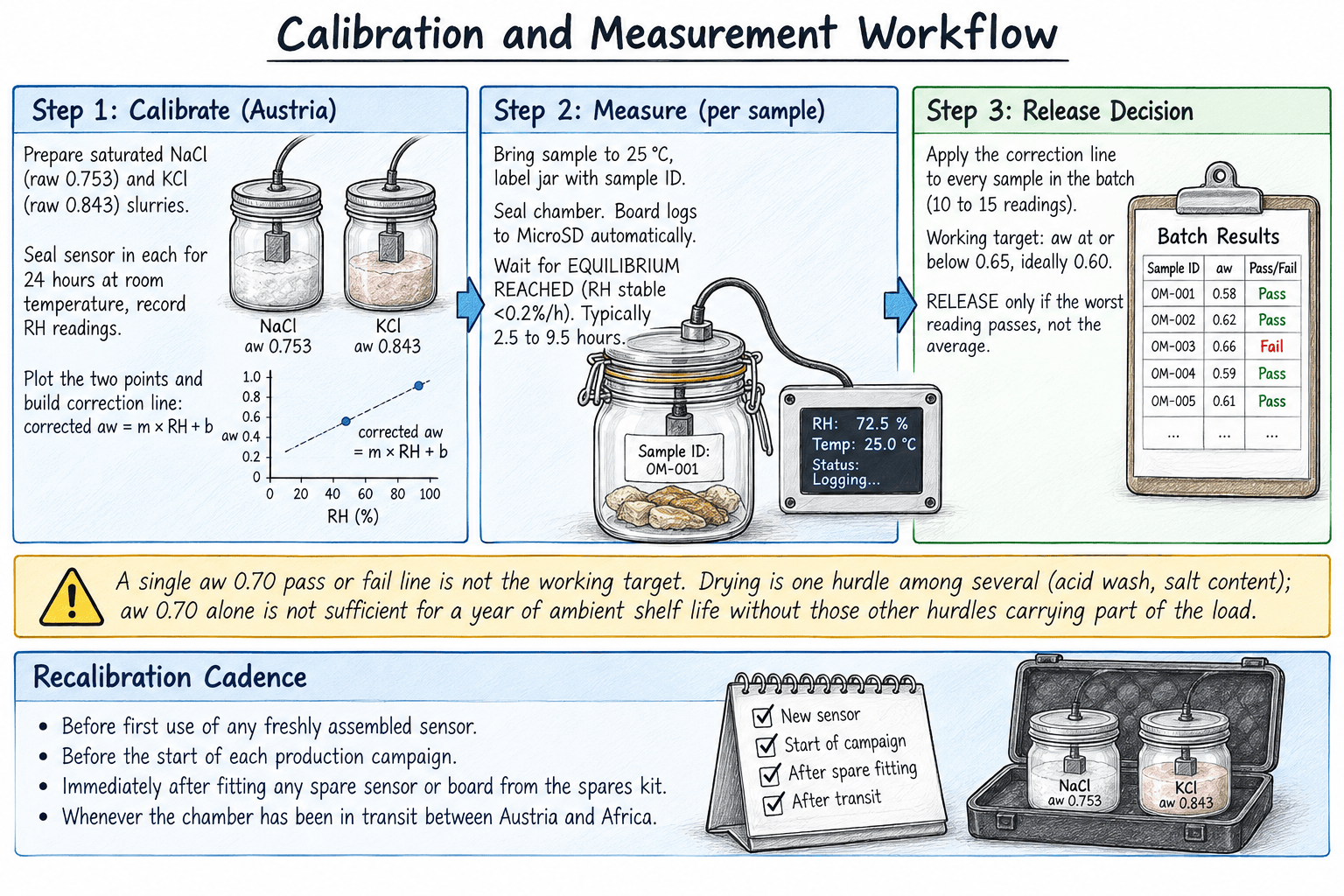
This is not a one time step done only in Austria before travel. Calibration should be repeated whenever the sensor or board is swapped for a spare, and again once the unit arrives in Africa, since handling and transit can shift a sensor’s reading even when nothing is visibly wrong with it. A working rule is to recalibrate before the start of each production campaign, and immediately after fitting any spare sensor or board from the spares kit, rather than assuming the last calibration still holds.
Calculating the Two-Point Linear Correction Line
The steps below use saturated NaCl and KCl reference slurries to build the correction line applied to every raw sensor reading.

Daily Logging Without a Network Connection
The board logs directly to a MicroSD card rather than over WiFi. Every equilibrium result the algorithm confirms, sample ID, time to plateau, corrected aw, and the readings leading up to it, is written straight to a CSV file on the card as it happens. This removes any dependence on factory WiFi, which cannot be assumed reliable, and gives a physical, auditable record with nothing between the reading and the file.
At the end of the day the card is pulled and its contents copied to a laptop, either by reading the card directly or connecting the board by USB cable. The file already contains every result the chamber declared complete that day. No analysis is required at this point, since the plateau has already been identified by the device itself, not judged afterward from raw numbers on a spreadsheet.
Running more than one chamber at a time is how a daily sampling programme should work in practice. Two or three jars, loaded with pieces cut from different parts of the same batch, thicker sections and thinner sections included, run and log independently through the day or overnight. Each writes to its own card, or to separate files on a shared card if the chambers are wired to a single board, tagged by sample ID so the results are never mixed up. This gives a spread of readings per batch rather than a single spot check, more informative for a tissue as uneven as omasum than for a more uniform product, at no additional operator time beyond loading the extra jars.
Networked Logging: WiFi and Satellite as an Alternative to the MicroSD Card
The MicroSD approach was chosen because ordinary factory WiFi in the regions this system will operate in cannot be assumed reliable, and a measurement system that depends on a network connection to save its result is a fragile design. That reasoning still holds as the default. The Feather HUZZAH ESP8266 already specified has WiFi built in, so a networked alternative needs a firmware change, not a new part.
Satellite internet is a genuine change to the reliability picture in parts of Africa where fixed line and mobile broadband infrastructure is weak. In Nigeria specifically, Starlink is already commercially available, with a standard hardware kit currently priced at roughly 590,000 to 669,000 naira, approximately 384 to 435 euros at the prevailing exchange rate, and a residential subscription from roughly 57,000 naira a month, approximately 37 euros, rising to roughly 159,000 naira a month, approximately 103 euros, for the business priority tier aimed at users who cannot tolerate congestion related slowdowns. Coverage and plan availability vary by state and by how congested the local residential tier already is, and prices in naira terms have moved more than once within 2026, so current figures should be checked directly against the Starlink website for the specific site before budgeting against them.
A sensible design keeps the MicroSD card as the permanent, always-on record, exactly as built, and adds networked reporting as an optional extra on top of it rather than a replacement for it. When a WiFi network is present, whether an ordinary factory router or one fed by a satellite terminal, the board pushes each completed reading to a central server or a cloud spreadsheet at the moment the display shows EQUILIBRIUM REACHED. When no network is present, or the push fails, the reading still exists on the card as it does today, and nothing is lost. This costs almost nothing extra in hardware, since the WiFi radio is already on the board, and the main addition is a small piece of firmware logic and, if satellite connectivity is the chosen route, the satellite terminal itself at the factory level, shared across every chamber on site rather than purchased per chamber.
What Setting This Up Would Require
- A network at the factory site. This can be an ordinary WiFi router if the site already has reliable fixed line or mobile broadband, or a satellite terminal such as a Starlink kit feeding a local router where fixed infrastructure is weak or absent.
- A firmware update to the existing board. The ESP8266 already used for the display and MicroSD logging is added to the local WiFi network with a network name and password, and the code is extended to send each completed reading, sample ID, time to plateau, and corrected aw, to a server address whenever a connection is available.
- Somewhere for the data to land. This can be as simple as a shared spreadsheet reachable through a scripting service, or a small self-hosted database on a low cost server, depending on how many sites and chambers need to report into one place.
- A fallback rule in the firmware. If the network push fails or times out, the board must still complete the MicroSD write exactly as it does today, so a network outage during a run degrades the system to its current, already validated behaviour rather than losing the reading.
A Simple Program to Interpret the Downloaded Data
The CSV files pulled from the card, or received over the network under the option above, are plain rows of sample ID, time to plateau, corrected aw, and a timestamp. Reading them by eye across several chambers and several days quickly becomes tedious and error prone, so a short summary script earns its place from the outset rather than being added later once the volume of files has grown. The outline below is deliberately simple, reads every CSV file in a folder, groups the readings by batch, and reports whether the batch passes the working target, using the maximum reading in the batch as the deciding figure rather than the average, in line with the release rule set out in the next section.
Python outline, aw_batch_report.py
import csv, glob, statistics
TARGET_AW = 0.65 # working target, adjust once validation locks a final figure
BATCH_FIELD = “sample_id” # sample IDs are expected in the form BATCH-PIECE, e.g. B240914-03
readings = {}
for path in glob.glob(“*.csv”):
with open(path, newline=””) as f:
for row in csv.DictReader(f):
batch = row[BATCH_FIELD].split(“-“)[0]
readings.setdefault(batch, []).append(float(row[“corrected_aw”]))
for batch, values in sorted(readings.items()):
worst = max(values)
status = “PASS” if worst <= TARGET_AW else “HOLD, retest or continue drying”
print(f”{batch}: n={len(values)} mean={statistics.mean(values):.3f} “
f”max={worst:.3f} target={TARGET_AW} {status}”)
This is a starting point, not a finished tool. It assumes sample IDs are written in a batch-then-piece format at Step 3 of the operator procedure, for example B240914-03 for the third piece cut from a batch dried on the 14th of September. Extending it to flag any sample still short of EQUILIBRIUM REACHED, to plot the log against the date, temperature, and drying time relationship described earlier, or to write a batch report file automatically, are all reasonable next steps once the basic version has been used on real data for a few production cycles.
Operator Procedure: Measuring a Batch After Calibration
This procedure uses the working draft values developed for this guide. They are starting points for a validation trial, not settled figures. Once a trial confirms them against a reference instrument, they should be locked into the final SOP.
Step 1. Bring the Sample to Temperature Before Sealing
Do not place a sample straight from cold storage into the chamber. Let it warm up first.
If a probe thermometer is available, push it into the thickest part of the sample and wait for the reading to settle. Seal the sample into the chamber once the probe reads close to 25 degrees Celsius, the chamber’s working temperature in the draft procedure, within about 1 degree Celsius as a practical target.
If no probe is available, let the sample sit out until it feels like room temperature to the touch, no longer cool or cold. This is a rougher check than a probe reading, so it should only be used as a fallback, not the default method.
Either way, a cold sample sealed into a warm chamber gives a false reading. A 0.1 degree Celsius gap between the sample and the headspace air can shift the measured water activity by roughly 0.005, enough to move a reading near 0.700 across the line between pass and fail. Where the target specification sits close to 0.700, getting the sample to temperature first is not optional.
Step 2. Cut the Sample the Same Way Every Time
The piece must be taken from the same anatomical location on the omasum each time, cut to the same approximate size, and loaded into the chamber within a fixed, short window after cutting, no more than two or three minutes as a working default. The sample must not be minced to speed up the reading. Mincing generates heat and exposes moisture that would not normally be exposed, changing what is actually being measured. Until a validation trial sets the final sample mass, piece count, and cutting method, the preparation used for each trial run should be recorded so results can be compared against each other.
Step 3. Label the Jar, Seal the Chamber, and Start the Run
Before sealing, write the sample ID on the jar itself, tying it to the batch it was cut from. Once sealed, the display shows MEASURING along with the current RH and temperature, and the board begins writing readings to the MicroSD card under that sample ID automatically. The MEASURING figure on the display is not the number to record. It only confirms the chamber is running and logging.
Step 4. Watch for the RH CHANGE DETECTED Signal
While the reading is still moving, the display shows RH CHANGE DETECTED alongside the live figures. As a working starting rule, the reading is treated as still moving if RH shifts by more than 0.2 percent within a one hour window. Nothing needs to be written down at this stage. The card is already logging every reading in the background.
Step 5. Confirm the Plateau Before Trusting a Result
A typical equilibration run, shown here as an illustrative example rather than measured omasum data, looks like this.
| Elapsed time | Headspace RH | Raw aw |
| 0 hours | 55.0 percent | 0.550 |
| 1 hour | 62.0 percent | 0.620 |
| 2 hours | 66.0 percent | 0.660 |
| 4 hours | 68.5 percent | 0.685 |
| 6 hours | 69.6 percent | 0.696 |
| 8 hours | 70.1 percent | 0.701 |
| 10 hours | 70.3 percent | 0.703 |
| 12 hours | 70.3 percent | 0.703 |
| 14 hours | 70.3 percent | 0.703 |
The pattern to recognise is fast movement early, a slowing rate through the middle hours, and a flat line at the end. In this illustrative case the flat line starts around hour ten and holds through hour fourteen. Actual plateau time will vary with piece thickness and how salt and moisture are distributed through the sample, which is why the flat line, not the clock, decides when the reading is finished.
Step 6. Let the Display Confirm Equilibrium, Then Move On
Once both temperature and RH have held within their validated tolerance for the required observation window, the display switches automatically to EQUILIBRIUM REACHED, showing the stable RH, the stable temperature, and the corrected aw, and the card records this final result against the sample ID. Nothing needs to be copied down by hand at this point. If the display still shows MEASURING or RH CHANGE DETECTED, the reading is not finished, regardless of elapsed time, and the jar should be left running.
Calibration and Testing Schedule for a One Tonne Batch
The preceding sections describe calibration and per-sample measurement separately. This section ties them together into the schedule that actually runs against a single one tonne batch on the production floor.
Before the Batch Starts
- Confirm calibration status of every chamber that will be used. If this is the first batch of a new production campaign, or any sensor or board has been swapped since the last calibration, run the two point NaCl and KCl calibration described earlier before touching the batch.
- Confirm the probe thermometer and the log from the previous batch are on hand, since these are what will indicate when the batch is approaching target, not a fixed number of drying days.
During Drying
- Take probe thermometer readings at multiple points through the stack daily, without opening a sealed aw chamber for every check.
- Compare the day’s conditions and elapsed time against the date, temperature, and drying time log built from previous batches, to judge when this batch is likely approaching target.
Once the Batch Is Judged Close to Target
- Pull 10 to 15 samples, weighted toward the thickest and most folded sections, from different locations, thicknesses, and positions in the salting stack.
- Run each sample through a calibrated chamber following Steps 1 to 6 of the operator procedure above, labelling each with a sample ID that ties it to this batch.
- Let every chamber reach EQUILIBRIUM REACHED before reading it. A jar still showing MEASURING or RH CHANGE DETECTED at the end of the day is left running rather than treated as failed or skipped.
The Release Rule
A batch is released once every one of its 10 to 15 samples reads at or below the working target aw, not once the average of the set does. The worst reading in the batch, not the mean, is what decides the outcome, because the average can hide a single under-dried piece from the thickest section, and that piece is the one that determines whether the batch is actually shelf stable. If any sample exceeds target, the batch continues drying and the sampling step is repeated, weighted again toward the sections that failed, rather than being released on the strength of the samples that already passed.
How the Data Is Used
Each completed reading in the CSV file carries a sample ID, a time to plateau, and a corrected aw. On its own, a single reading answers one question, whether that piece sits above or below the working target on the day it was cut. Read across a full day, the 10 to 15 readings from a batch answer the release question for that batch, weighted toward the thickest and most folded sections that are the last to reach target. Read across many days, the same log becomes the input for the date, temperature, and drying time relationship described earlier, letting the expected time to target for a given week’s conditions be predicted with more confidence as more cycles are recorded.
What Remains Open Until Validation Is Complete
The 0.2 percent per hour stability rule, the exact sample mass and piece count, and the expected plateau time for omasum are draft figures pending confirmation. Until 10 to 20 trial runs have been compared against a recognised reference water activity instrument and agreement has been demonstrated, every reading from this chamber should be treated as a screening result, useful for checking whether a batch sits above or below the working target, not as a certified figure for a compliance document. The calibration itself is part of this validation. A correction line that has not been rechecked since the last sensor swap or the last transit between Austria and Africa should not be assumed to still be accurate.
Economic Review: Shelf-Stable Product and Measurement System Choice
Avoiding the Cold Chain Premium
Reefer ocean freight commands a structural rate premium over an equivalent dry container on the same route, commonly cited at 50 to 100 percent above the dry rate, rising further during peak season or on lanes where reefer flows are imbalanced [7]. This premium exists because the equipment costs more to own, maintain, and repair than a standard dry box, and requires power and monitoring throughout the voyage, so it persists in stable freight markets and is not simply a symptom of temporary tightness [7]. A shelf-stable, ambient omasum shipment avoids this premium entirely, avoids the added handling and terminal costs reefer cargo attracts, and avoids the single point of failure risk that a multi week ocean voyage under refrigeration carries, where one equipment failure or one missed reefer plug at a transhipment port can spoil an entire container.
What This Means in Practice, at Container Scale
Using the working estimate of approximately 13 euro cents per kilogram saved by selling omasum ambient rather than refrigerated, a 28 tonne container, 28,000 kilograms, saves approximately 3,640 euros against the refrigerated equivalent. Against a container sold at 5 euros per kilogram, a sale value of approximately 140,000 euros, that saving represents approximately 2.6 percent of sale value, realised without any change to the product’s formulation, its selling price, or the volume moved. This figure is Eben van Tonder’s own working estimate for this guide, not an independently documented breakdown of reefer premium, cold storage cost, and spoilage risk avoided, and it would be strengthened by attaching a costed breakdown of what the 13 cents actually covers on the specific trade lanes used.
DIY Measurement System Versus a Fully Commercial Setup
The same logic that favours ambient shipping over refrigerated shipping favours the DIY measurement system over an all-commercial one, for the same underlying reason, a large recurring cost is avoided by substituting a cheaper method that still does the job once properly validated. One reference instrument plus three DIY chambers with spares comes to roughly 2,300 to 2,700 euros as a starting outlay. Matching that same validation and screening capacity using commercial meters alone would cost three to four times as much, since each additional commercial unit runs close to the reference instrument’s own price, roughly 1,700 euros, while each additional DIY chamber for scaling up daily screening costs roughly 150 to 200 euros. Scaling to, for example, six chambers to cover higher batch volume would cost roughly 900 to 1,200 euros the DIY way against roughly 10,200 euros the fully commercial way for the equivalent count, a gap that widens every time capacity is added rather than narrowing.
The two economic arguments in this guide are independent of each other and both real. The 13 cents per kilogram figure is a saving in how the finished product is shipped and stored. The DIY versus commercial instrument comparison is a saving in how the finished product is tested before it is allowed to be called shelf stable in the first place. Neither substitutes for the other, and the second is what makes the first defensible, since a shelf-stable claim that cannot be backed by a properly calibrated aw reading on every batch is a liability, not a saving.
References
[1] Beuchat, L.R. (1983). Influence of water activity on growth, metabolic activities and survival of yeasts and molds. Journal of Food Protection, 46(2), 135 to 141.
[2] Petit, T., Caro, Y., Petit, A.-S., Santchurn, S.J., Collignan, A. (2014). Physicochemical and microbiological characteristics of biltong, a traditional salted dried meat of South Africa. Meat Science, 96(3), 1313 to 1317. https://doi.org/10.1016/j.meatsci.2013.11.003
[3] Jones, M., Arnaud, E., Gouws, P., Hoffman, L.C. (2017). Processing of South African biltong, a review. South African Journal of Animal Science, 47(6), 743 to 757. https://doi.org/10.4314/sajas.v47i6.2
[4] Jones, M., Arnaud, E., Gouws, P., Hoffman, L.C. (2019). Effects of the addition of vinegar, weight loss and packaging method on the physicochemical properties and microbiological profile of biltong. Meat Science, 156, 214 to 221. https://doi.org/10.1016/j.meatsci.2019.06.003
[5] Leistner, L., Gorris, L.G.M. (1995). Food preservation by hurdle technology. Trends in Food Science and Technology, 6(2), 41 to 46. https://doi.org/10.1016/S0924-2244(00)88941-4
[6] Leistner, L. (2000). Basic aspects of food preservation by hurdle technology. International Journal of Food Microbiology, 55(1 to 3), 181 to 186. https://doi.org/10.1016/S0168-1605(00)00161-6
[7] HZ Containers (2026). Reefer container vs. dry container, the ultimate guide to their differences. Industry resource, accessed September 2026. https://hz-containers.com/en/news/reefer-container-vs-dry-container-the-ultimate-guide-to-their-differences/
[8] Starlink Nigeria pricing, cross checked across multiple reseller and news sources current to March to August 2026, converted at the prevailing NGN to EUR exchange rate of approximately 1 EUR = 1,537 NGN, September 2026. Current figures should be verified directly at starlink.com before budgeting against them.
[9] Scott, W.J. (1953). Water relations of Staphylococcus aureus at 30 degrees C. Australian Journal of Biological Sciences, 6(4), 549 to 564. https://doi.org/10.1071/BI9530549
[10] Van Tonder, E., Van Tonder-Berger, C. (2026). Dry Salted Beef Omasum Production. Earthworm Express, 19 September 2026. https://earthwormexpress.com/the-meat-factory/meat-science-research/dry-salted-beef-omasum-production/
Reference [8] is a commercial pricing source rather than a peer reviewed one, included because the WiFi and satellite section above depends on it directly. Reference [10] is the author’s own companion production guide, linked because it is where the wider hurdle system and the water activity target this document measures against are set out in full. All other references are peer reviewed journal articles or the standard hurdle technology and water activity literature. Figures attributed to Eben van Tonder in the Executive Summary and the Economic Review, the 13 euro cents per kilogram saving specifically, are the author’s own working estimates for this guide and are not independently sourced here.